Column Definition Tab (New Calculated Column)
This feature allows you to create a new column based on a
formula.
Calculated columns are useful in data analysis; for example,
you might define a column that is the derivative of another column with
respect to time, a smoothed version of a sensor column, or the ratio of
two sensor columns. Calculated columns can be graphed or used in
further analysis.
The new calculated column can be a function of another column
or columns, or it may be defined by a rule that does not depend on
other columns. Arithmetic operators ("^", "*", "/", "+", "-"),
parentheses, and other mathematical functions can be used to create a
new column based on one or more existing columns. For example, if you
have current and potential data, you can use a new column to calculate
the power (current times potential). This definition is shown here.
You can create a calculated column by choosing New
Calculated Column from the Data menu. You
can edit calculated columns by either double-clicking the column name
in the data table or choosing Column
Options from the Data menu.
Labels and Units
Name
The long name is used in graph axis labels, column headings
and menus whenever there is sufficient room. You cannot use a quotation
character (“) in the Name.
Short Name
The Short Name is used in graph axis
labels, column headings, and menus whenever there is limited room. If
you do not enter a Short Name, the first letter of the Name will be
used.
Units
The Unit follows the Name in graph axis
labels and column headings. If the units that you enter are not the
same as a visible line on the active graph window, you will be warned
that your column will not be automatically shown in the graph. You can
either re-enter units that match a visible line, or click on the y-axis
label in the graph window and select your column to be drawn.
You can choose special symbols
(including subscripts and superscripts) to be included in all of the
above fields by clicking  .
.
Destination
A Calculated Column resides in a particular Data Set.
Choose which Data Set will receive the new column. If Add to
All Similar Data Sets, is checked, copies of the calculated
column will be added to Data Sets that share the same column names. For
example, you might want to create a smoothed version of the data from
an accelerometer, and you want such a column in each of your stored
runs. To do this, add a calculated column to the Latest Data Set, and
check Add to All Similar Data Sets to add to all
similar data sets.
Equation
Equations can contain column names, mathematical functions,
constants, and parameters.
If you want your equation to include data from a column, you can choose
column names from the Variables (Columns)
drop-down menu or you can type existing column names (inside quotation
marks). If you choose a sensor column as a variable, a Display
During Live Readouts checkbox will appear. If you select this
option, the readouts for the calculated column will be displayed on the
toolbar.
You may also enter mathematical functions by choosing them
from the Functions drop-down menu or by typing them
(see below for function definitions). For example, if you have a column
named "X", and you want to create a column whose values are the square
roots of the values in "X", select sqrt() from the Functions
menu, then select X from the Variables
(Columns) menu. Your equation would look like this:
sqrt("X")
Let's suppose you named your new column "Root". If "X" had the
values: 4, 25, and 64, then "Root" would have the values: 2, 5, and
8. If you changed any of the values in "X", "Root" would also
change. "Root" is linked to and dependent on the column "X".
If you delete "X", "Root" will also be deleted.
Mathematical functions can be used alone or in combination
with others; you can nest functions, use arithmetic operators inside
functions, and use parentheses to group operations. For example, a
valid expression (assuming you have columns named "X" and "Y"), is:
sin(("X" + "Y") / sqrt(3))
If the the equations are not mathematically legal (e.g. square
roots of negative numbers), a blank cell will be displayed. Any further
expression based on that cell will also result in a blank cell.
To insert a specific parameter
into a calculated column's equation, select its name from the Parameters
drop-down menu. A parameter is a place to store an adjustable numeric
value. The parameter can be referred to in calculated columns, trigger
level thresholds, and similar fields.
Column Selection with Multiple Data Columns
When you include a column as part of an equation, you can
enter only the column name or you can enter the full name. The full
name specifies the data set and the column name (for example, Run 1 |
Time). The difference is subtle but can be useful. When you enter just
the column name, you are saying that you want the calculated column to
use a column of that name in the data set in which the calculated
column is located. When you give the full name, you are referring to a
specific column in a specific data set, regardless of in which data set
you have placed your calculated column.
For example, let's say you have two sets of data that each
contain 3 columns: X, Y, and a calculated column called CC. If the CC
equation is "X" + "Y", the values in the Run 1 calculated column will
be the sum of Run 1 X and Run 1 Y and the values in the Run 2
calculated column will be the sum of Run 2 X and Run 2 Y. However, if
the CC equation is "Run 1 | X" + "Y", Run 1 CC will be the sum of Run 1
X and Run 1 Y and Run 2 CC will be the sum of Run 1 X and Run 2 Y. To
select the full name, choose Variables (Columns) >
Choose Specific Column.
Functions
- Trigonometric functions will use degrees or radians as set
in the Settings for (file
name) in the File menu.
Function
|
Description
|
analysis >
|
|
analysis
|
("X", startRow, endRow)
Takes all columns named "X" and extracts startRow to endRow for each of
those columns, appending the values into a single column. |
dataSets
|
datasets("X")
Appends the dataset names of all datasets that have a column named "X".
Use analysis and datasets together to create a graph (analysis on the
vertical axis and datasets on the horizontal). for example, if you had
3 datasets as follows:
DS1 DS2 DS3
X X
Y
1 11
21
2 12
22
and then added analysis("X", 1, 1) and datasets("X") you would get:
datasets analysis
DS1
1
DS2
11
|
beats per minute
|
BeatsPerMinute("Signal", "Time", intervalInSeconds,
minPercent, maxPercent, noise)
Returns the number of beats per minute of the values in "Signal" vs.
"Time". This function is similar to the rate function except that the
interval given here is always in seconds and the returned value is
always in minutes. For example, if "Time" is in seconds then:
beatsPerMinute("Signal", "Time", interval, min, max, noise) = 60 *
rate("Signal", "Time", interval, min, max, noise)
|
blood pressure >
|
|
diastolic
|
The measured arterial pressure when the heart is at
rest. "Pressure" and a "Time" column as inputs and return a single
number.
diastolic("Pressure", "Time")
"Pressure": Pressure values from the BPS
"Time": Time the pressure values were recorded
Returns the smaller number of blood pressure
|
meanArterialPressure
|
meanArterialPressure("Pressure", "Time")
"Pressure": Pressure values from the BPS
"Time": Time the pressure values were recorded
Returns the pressure value at the max peak used for blood pressure
calculations.
|
Oscillations
|
Oscillations("Pressure", "Time")
"Pressure": Pressure values from the BPS
"Time": Time the pressure values were recorded
Returns the Oscillations of the peaks and valleys used to calculate
systolic and other blood pressure values.
|
OscillatoryPeaks
|
OscillatoryPeaks("Pressure", "Time")
"Pressure": Pressure values from the BPS
"Time": Time the pressure values were recorded
Returns the peaks used to calculate systolic, diastolic, and pulse (the
"high" values in "Oscillations"). |
pulse
|
pulse("Pressure", "Time")
"Pressure": Pressure values from the BPS
"Time": Time the pressure values were recorded
Returns the pulse using the inputs from the Blood Pressure Sensor
(similar results, different algorithm as the other beats-per-minute
functions)
|
systolic
|
systolic("Pressure", "Time")
"Pressure": Pressure values from the BPS
"Time": Time the pressure values were recorded
The measured arterial pressure when the heart contracts. Returns the
larger number of blood pressure
|
boolean >
|
For the boolean functions a 1 is considered true, 0
false and anything else an invalid input |
AND
|
AND(X, Y) return 1 if and only if X and Y are both 1 |
NOT
|
NOT(X) return 1 if
X is 0; 0 if X is 1 |
OR
|
OR(X, Y) return 1 if X or Y is 1 |
XOR
|
XOR(X, Y) return 1 if X or Y is 1 but not both |
calculus >
|
|
derivative
|
derivative("Y", "X")
"Y": A column of real numbers
"X": Optional. A column of real numbers
The numerical derivative is the weighted average of the slope of 'n'
points around each point. You can set 'n' in Settings for (Name).
If you don't supply an "X" column, the program will find one. |
derivativeSG
|
derivativeSG("Y", "X")
"Y": A column of real numbers
"X": Optional. A column of real numbers
Savitsky-Golay derivative. Fits a polynomial to 'n' points around each
point and computes the derivative of the polynomial at that point. You
can set 'n' in Settings
for (Name). If you don't supply an "X" column, the program
will find one. |
derivativeTimeShift
|
derivativeTimeShift("Y", "X")
Returns the derivative of "Y" with respect to "X".
This function is specifically designed to be used with photogate and
picket fence data. The derivatives returned are adjusted to estimate
values at the start of the timing interval, instead of the midpoint.
For details see The Physics Teacher, Vol 35, April 1997, p. 220. The
article written by William Leonard is entitled "The Dangers of
Automated Data Analysis."
Average velocity during the time interval is equal to the instantaneous
velocity at midpoint of the time interval.
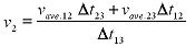
Where
 |
integral
|
integral("Y","X")
"Y": A column of real numbers
"X": Optional. A column of real numbers
The numerical integral is the running sum of the areas of rectangles
calculated by the midpoint rule. The i'th rectangle is (Yi - Y(i-1)) /
(Xi - X(i-1)). If you don't supply an "X" column, the program will find
one. |
secondderivative
|
secondDerivative("Y", "X")
"Y": A column of real numbers
"X": Optional. A column of real numbers
Calculates the numerical second derivative of "Y" with respect to "X".
If you don't supply an "X" column, the program will find one. |
secondderivativeSG
|
secondDerivativeSG("Y", "X")
"Y": A column of real numbers
"X": Optional. A column of real numbers
Savitsky-Golay second derivative. Fits a polynomial to 'n' points
around each point and computes the second derivative of the polynomial
at that point. You can set 'n' in Settings
for (Name). If you don't supply an "X" column, the program
will find one. |
secondderivative
Time Shift
|
secondDerivativeTimeShift("Y", "X")
"Y": A column of real numbers
"X": Optional. A column of real numbers
Numerical time-shifted second derivative. Calculates the second
numerical derivative of "Y" with respect to "X". The values are shifted
so that the derivatives are calculated at the midpoints between each
two values. If you don't supply an "X" column, the program will find
one.
 |
|
|
collapse("X")
Returns a column with all non-numerical cells (blanks and text) removed. |
collapseIndirect
|
collapseIndirect(X, Y)
Returns a column of only the rows in "X" corresponding to rows in "Y"
that have valid numerical cells. |
constant
|
Constant(x, num)
x: A real number
num: A real number or a column
Generates a constant column filled with the value 'x'. The
number of values in the returned column is num, or if a column was
passed in, the size of the passed-in column. |
delta
|
delta ("X")
"X": A column of real numbers
Returns a column of values where the i'th value is the i'th value in
"X" minus the (i-1)'th value in "X". |
digital filtering >
|
|
lowPassFilter
|
("Y", "X", "ripple", "freqCutoff")
"Y": The data column to be filtered
"X": The associated time column for "Y"
"ripple": The ripple allowed in the pass-band
"freqCutoff": Cut-off frequency (-3dB), in hertz
Applies a Chebyshev low-pass filter. For "ripple", enter a value that
is a percent of the pass-band. To apply a Butterworth low-pass filter,
set "ripple" to 0. |
highPassFilter
|
("Y", "X", "ripple", "freqCutoff")
"Y": The data column to be filtered
"X": The associated time column for "Y"
"ripple": The ripple allowed in the pass-band
"freqCutoff": Cut-off frequency (-3dB), in hertz
Applies a Chebyshev high-pass filter. For "ripple", enter a value that
is a percent of the pass-band. To apply a Butterworth high-pass filter,
set ripple to 0. |
bandPassFliter
|
("Y", "X", "lowFreq", "highFreq")
"Y": The data column to be filtered
"X": The associated time column for "Y"
"lowFreq": Low frequency cut-off (-3dB), in hertz
"highFreq": High frequency cut-off (-3dB), in hertz
Ripple is automatically set to zero and is not adjustable. The function
returns the signal with the frequencies outside the designated
frequency range removed. |
bandStopFliter
|
("Y", "X", "lowFreq", "highFreq")
"Y": The data column to be filtered
"X": The associated time column for "Y"
"lowFreq": Low frequency cut-off (-3dB), in hertz
"highFreq": High frequency cut-off (-3dB), in hertz
Ripple is automatically set to zero and is not adjustable. The function
returns the signal with the frequencies inside the designated frequency
range removed. |
timeDecayFilter
|
("Y", "X", "decayConstant")
"Y": The data column to be filtered
"X": The associated time column for "Y"
"decayConstant": A value in seconds that determines the decay of "Y"
Applies an exponential time decay to the signal. |
ElectrophoresisInterpolate
|
ElectrophoresisInterpolate("Std. Dist", "Std. BP",
"Dist")
"Std. Dist": Distances from the standard
"Std. BP": Base Pair Counts from the standard
"Dist": Distances to interpolate
Returns a column of base pair counts based on the Electrophoresis curve
fit for "Std. Dist" vs. "Std. BP" given "Dist". Will NOT work if curve
fit has been deleted. This function is used automatically when doing a
Gel Analysis (Electrophoresis).
|
exp
|
exp("X")
"X": A column of real numbers
Returns the exponent, exp(x) = e^x, where e is the natural log base
(2.17...). |
integer
|
integer("X")
Extracts the integral part of values in "X". |
interpolate
|
interpolate("X")
Fills in missing values using linear interpolation. |
ln
|
ln("X")
"X": A column of real numbers larger than 0
Returns the natural logarithm. If b = ln(a) then e^b = a
(Where e is the constant 2.17...). |
log
|
log("X")
"X": A column of real numbers larger than 0
(Log base 10) If b = log(a) then 10^b = a. |
modulo
|
modulo("X", n)
"X": A column of integers
n: An integer larger than 0
Returns the remainder of each of the numbers in "X" when divided by n. |
|
|
|
Blocked MidTimes
|
BlockedMidTimes("Time", "Gate1", "Gate2")
"Time": Optional. A column of real numbers (the times of events)
"Gate1": A column of photogate states (1's and 0's)
"Gate2": Optional. A column of photogate states (1's and 0's)
Calculate the average times between blocked events from Gate 1 to Gate
2. If you don't enter a "Time" column, the program will find one. If
you don't enter "Gate2", "Gate1" will be used. |
Blocked to Blocked
|
BlockedToBlocked("Time", "Gate1", "Gate2")
"Time": Optional. A column of real numbers (the times of events)
"Gate1": A column of photogate states (1's and 0's)
"Gate2": Optional. A column of photogate states (1's and 0's)
Returns a column of the times between successive blocked events in gate
1 and blocked events in gate 2. If you don't enter a "Time" column, the
program will find one. If you don't enter "Gate2", "Gate1" will be
used. |
Blocked to Unblocked
|
BlockedToUnblocked("Time", "Gate1", "Gate2")
"Time": Optional. A column of real numbers (the times of events)
"Gate1": A column of photogate states (1's and 0's)
"Gate2": Optional. A column of photogate states (1's and 0's)
Returns a column of the times between successive blocked events in gate
1 and unblocked events in gate 2. If you don't enter a "Time" column,
the program will find one. If you don't enter "Gate2", "Gate1" will be
used. |
Blocked to Unblocked MidTimes
|
Blocked to Unblocked MidTimes
"Time": Optional. A column of real numbers (the times of events)
"Gate1": A column of photogate states (1's and 0's)
"Gate2": Optional. A column of photogate states (1's and 0's)
Calculate the average time between the blocked events in gate 1 and
unblocked events in gate 2. If you don't enter a "Time" column, the
program will find one. If you don't enter "Gate2", "Gate1" will be
used. |
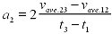
derivativeTimeShift
|
DerivativeTimeShift ("Y", "X")
Returns the derivative of "Y" with respect to "X".
This function is specifically designed to be used with photogate and
picket fence data. The derivatives returned are adjusted to estimate
values at the start of the timing interval, instead of the midpoint.
For details see The Physics Teacher, Vol 35, April 1997, p. 220.
Average velocity during the time interval is equal to the instantaneous
velocity at midpoint of the time interval.
Where
|
Pendulum Period
|
PendulumPeriod("Time", "Gate1")
"Time": Optional. A column of real numbers (the times of events)
"Gate1": A column of photogate states (1's and 0's)
Calculate the time between every other blocked event on Gate 1. If you
don't enter a "Time" column, the program will find one. |
secondDerivativeTimeShift
|
secondDerivativeTimeShift("Y", "X")
"Y": A column of real numbers
"X": Optional. A column of real numbers
Numerical time-shifted second derivative. Calculates the second
numerical derivative of "Y" with respect to "X". The values are shifted
so that the derivatives are calculated at the midpoints between each
two values. If you don't supply an "X" column, the program will find
one.
|
Unblocked to Blocked
|
UnblockedToBlocked("Time", "Gate1", "Gate2")
"Time": Optional. A column of real numbers (the times of events)
"Gate1": A column of photogate states (1's and 0's)
"Gate2": Optional. A column of photogate states (1's and 0's)
Returns a column of the times between successive unblocked events in
gate 1 and blocked events in gate 2. If you don't enter a "Time"
column, the program will find one. If you don't enter "Gate2", "Gate1"
will be used. |
Unblocked to Unblocked
|
UnblockedToUnblocked("Time", "Gate1", "Gate2")
"Time": Optional. A column of real numbers (the times of events)
"Gate1": A column of photogate states (1's and 0's)
"Gate2": Optional. A column of photogate states (1's and 0's)
Returns a column of the times between successive unblocked events in
gate 1 and unblocked events in gate 2. If you don't enter a "Time"
column, the program will find one. If you don't enter "Gate2", "Gate1"
will be used. |
Unblocked to Blocked MidTimes
|
Unblocked to Blocked MidTimes
"Time": Optional. A column of real numbers (the times of events)
"Gate1": A column of photogate states (1's and 0's)
"Gate2": Optional. A column of photogate states (1's and 0's)
Calculate the average time between unblocked events in gate 1 and
blocked events in gate 2. If you don't enter a "Time" column, the
program will find one. If you don't enter "Gate2", "Gate1" will be
used. |
Unblocked MidTimes
|
UnblockedMidTimes("Time", "Gate1", "Gate2")
"Time": Optional. A column of real numbers (the times of events)
"Gate1": A column of photogate states (1's and 0's)
"Gate2": Optional. A column of photogate states (1's and 0's)
Calculate the average times between unblocked events from Gate 1 to
Gate 2. If you don't enter a "Time" column, the program will find one.
If you don't enter "Gate2", "Gate1" will be used. |
rate
|
rate("Y", "X", t, m1, m2, n)
"Y": A column of real numbers
"X": Optional. A column of real numbers
t: Optional. Time interval
m1: Optional. Minimum threshold
m2: Optional. Maximum threshold
n: Optional. Noise threshold
Returns the rate of "Y" with respect to "X", where t is the time
interval measured, m1 is min percentage threshold, m2 is max percentage
threshold, and n is noise threshold. "X", t, m1, m2, and noise are all
optional with default values "X" is time column, t = 1/10 the range, m1
= 40%, m2 = 60%, and noise = 0. Details
|
rotary motion >
|
|
amplitude
|
("Data Column", "Time Column", "Min Percent", "Max
Percent", "Time Interval")
"Data Column": Data for which you want to calculate amplitude
"Time Column": Associated time column for "Data Column"
"Min Percent": Threshold used to detect valleys
"Max Percent": Threshold used to detect peaks
"Time Interval": Period of time over which amplitude is calculated (in
the time units of the experiment)
Calculates peak to peak amplitude. For Min and Max Percent, enter
values between 0 and 100. Smaller values are more sensitive to noise
and thus more sensitive to real cycles. Larger values are less
sensitive to noise; too large of a value may filter out real cycles.
"Time Interval" ends at the row at which the value is calculated (the
current time). |
period
|
("Data Column", "Time Column", "Min Percent", "Max
Percent", "Time Interval")
"Data Column": Data for which you want to calculate period
"Time Column": Associated time column for "Data Column"
"Min Percent": Threshold used to detect valleys
"Max Percent": Threshold used to detect peaks
"Time Interval": Period of time over which period is calculated (in the
time units of the experiment)
Calculates the period of an oscillating function. For Min and Max
Percent, enter values between 0 and 100. Smaller values are more
sensitive to noise and thus more sensitive to real cycles. Larger
values are less sensitive to noise; too large of a value may filter out
real cycles. "Time Interval" ends at the row at which the value is
calculated (the current time). |
round
|
round("X")
"X": A column of real numbers
Round. Returns the closest integer to x. If x is equidistant to two
integers, round(x) gives the largest of the two (e.g., round(0.5) = 1).
|
smoothAve
|
smoothAve("X")
"X": A column of real numbers
Returns a column of moving averages of the values in "X". The width of
the "window" to use when averaging points can be set in Settings for (Name)...
|
statistics >
|
|
abs
|
abs("X")
"X": A column of real numbers
Absolute value. If x less than 0, then abs(x) = -x.
Otherwise, abs(x) = x. |
ceiling
|
ceiling("X")
"X": A column of real numbers
Returns the smallest integer larger than or equal to x. |
floor
|
floor("X")
"X": A column of real numbers
Returns the largest integer smaller than or equal to x. |
max
|
max("X")
"X": A column of real numbers
Compares all the values in a single column and returns a single
number-the largest number in the column. |
max2
|
max2("X", "Y")
"X": column of real numbers
"Y": A column of real numbers or a single number.
Compares all the values in a column against a real number (e.g
max2("X", 5.1)) |
mean
|
mean("X")
"X": A column of real numbers
Arithmetic mean. Returns the sum of all the values in "X" divided by
the number of values. |
median
|
Median("X").
"X": A column of real numbers
If m = median("X"), then half the numbers in "X" are greater than (or
equal) to m, and half are less than or equal. |
min
|
min("X")
"X": A column of real numbers
Compares all the values in a single column ,and returns a single
number-the smallest number in the column. |
min2
|
min("X", "Y")
"X": A column of real numbers
"Y": A column of real numbers or a single number
Compares all the values in a column against a real number (e.g
min2("X", 5.1))
|
numRows
|
NumRows("X")
"X": A column of real numbers
Returns a single value-the number of rows in the column. |
randInt
|
randInt(min, max, num):
min: A real number
max: A real number
num: A real number or a column
Random Integer. Returns a column of random integers between min and max
(inclusive). The size of the returned column is num. If num is a
column, then the size will be the number of rows in that column. |
randReal
|
randReal(min, max, num)
min: A real number
max: A real number
num: A real number or a column
Random Real. Returns a column of random real numbers between min and
max (inclusive). The size of the returned column is num. If num is a
column, then the size will be the number of rows in that column. |
stddev
|
stddev("X")
"X": A column of real numbers
Standard Deviation. Returns a column representing the standard
deviations of each of the numbers in a column. |
step
|
step(start, increment, num, first, skip)
start: Start value
increment: Increment value
num: Number of values to generate
first: Optional. First non-empty row
skip: Optional. Rows to skip between each value
Generates a column "num" rows long starting with "start" and
incrementing by "increment". "num" can be a positive integer or a
column name. Optional parameters: "first" is the first non-empty row
and "skip" is the number of rows to skip between each value. |
StepColumnBase
|
stepColumnBased("X", start, increment, first, skip)
start: Start value
increment: increment value
first: Optional. First non-empty row
skip: Optional. Row to skip between each value
Generates a column based on non-empty values in column "X" starting
with "start" and incrementing by "increment." "First" is the first
non-empty row and "skip" is the number of rows to skip between each
value. |
subset
|
subset("X", startRow, step)
"X": A column of real numbers
startRow: An integer larger than 0
step: An integer larger than 0
Extract a subset. Returns a column extracted from "X" starting with
'startRow' by 'step'. For example, subset("X", 1, 2) will get every
second row of "X" starting with row 1. |
sum
|
Sum("X")
"X": A column of real numbers
Returns a column whose n'th value is the sum of the values in "X" from
row 1 to n. |
sqrt
|
Square root. "X": A column of non-negative real
numbers.
If x is the square root of y, then x*x = y. |
trigonometric >
|
|
sin
|
sin("X")
"X": A column of real numbers
In a right triangle with angle between two sides 'x', sin(x) is the
length of the opposite side divided by the hypotenuse. |
cos
|
cos("X")
"X": A column of real numbers
In a right triangle with angle between two sides 'x', cos(x) is the
length of the adjacent side divided by the hypotenuse. |
tan
|
tan("X")
"X": A column of real numbers
In a right triangle with angle between two sides 'x', tan(x) is the
length of the opposite side divided by the adjacent side. |
asin
|
asin("X")
"X": A column of real numbers between -1 and 1
Arcsine function. asin(x) = the angle whose sine is x. |
acos
|
acos("X")
"X": A column of real numbers between -1 and 1
Arccosine function. acos(x) = the angle whose cosine is x. |
atan
|
atan("X")
"X": A column of real numbers
Arctangent function. atan(x) = the angle whose tangent is x. The result
will be between -pi/2 and pi/2. |
sinh
|
sinh("X")
"X": A column of real numbers
Hyperbolic sine. |
cosh
|
cosh("X")
"X": A column of real numbers
Hyperbolic cosine. |
tanh
|
tanh("X")
"X": A column of real numbers
Hyperbolic tangent. |
Value
|
Value(n, "X")
n: Number of rows backwards (when n < 0) or forwards (n
>0) in column "X" to extract a value from.
"X": Column from which to extract values .
Create a new column from another column by extracting offset values.
|
If data are imported from an experiment file, you may want to
specify the independent column. For example, if the imported data
included "time" in the first column but you wanted to calculate the
derivative of pH with respect to volume, you have to define the
derivative as derivative("pH","Volume").
See Also: